Day 0 Account Value: $2500 (+$0/0%)

After all of our preparation and research, today was the day I laid out the first trades of our little experiment, selling iron condors on GLD (gold ETF) and TLT (U.S. Treasury Bonds ETF). I’ll walk through the thought process for only the TLT iron condor as the GLD spread followed similar logic. After open and into the afternoon, I had charts for each of our Top 10 underlyings open in the template I described in the previous post and examined volatility. For each of the ten, I asked the following: is implied volatility high, low or mid-range compared to itself, and is there a strong divergence or convergence of implied and historical volatility?

For the equity index ETFs SPY, QQQ, and IWM, implied volatility is mid-range and 3-4% above 45-day historical volatility. For now, I’m not finding that particularly interesting and I’ll pass.

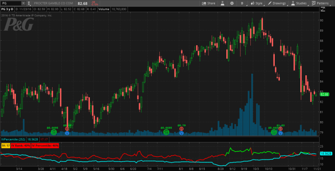
For our equity picks — AAPL, PG, BAC, FB, and BABA — implied volatility looks depressed (save PG at 60th percentile), but across the board is tracking historical volatility much tighter. An IV/HV spread of 1.1% on FB, for example, doesn’t give us much of an edge buying or selling volatility without trying to be predictive of the future. Keeping in line with our 30-60 day optimal expiry range, we’ll be looking at the Jan ’17 monthly options.

That left just two ETFs, GLD and TLT. Let’s examine the TLT setup:

At the time the trade was put on, TLT was trading with a 89th percentile IV and a 1.7% IV premium over HV. IV is certainly inflated compared to itself, but what about that IV/HV differential? Until I find a clean way to compare HV to itself, I have to rely on qualitatively interpreting the HV (blue) graph. A quick glance shows that HV is nearly as high as its been over the past year. With both IV and HV near the top of their ranges, I’m inclined to believe both will trend down towards their long-run averages and therefore sell volatility.

When selling volatility, we have a couple strategy choices, namely selling straddles, strangles, iron condors, ratio spreads, butterflies, or credit spreads. Straddles, strangles, and ratio spreads are short more contracts than they are long and are currently out of reach for our account size. That leaves iron condors (ICs), butterflies/iron flies, and credit spreads. Flies are great when IV is high as ATM options have the highest vega in the chain, but consequently carry more gamma risk. Credit spreads are simple and neat but also inherently carry more delta exposure than I’d like to start off. That leaves us with the IC.

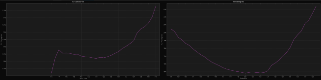
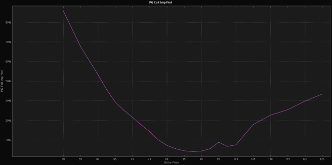
With our underlying and strategy selected, we can take a look at the volatility curve for calls and puts to help decide what strikes we want. With the ATM strikes being 120-121, we can see that ATM to near OTM volatility is fairly flat on the call side and sharper on the put side. Note how call IV doesn’t begin to ramp up until the $124 strike whereas put IV inflects ATM. This means the put strike selection will be more sensitive to volatility as we’ll be buying more volatility on the put side than call side, assuming we stay reasonably close to the money.

For the short strikes, I ended up choosing the closest to 30 delta, which were $117 and $124. This put me in a nice balance between taking in a decent credit and not having to pick long strikes that were too close in to avoid buying a lot of vol. On the long side I went with the $114 and $127 strikes, which happened to be in the 16-18 delta range. Any higher on the call side and I would have been buying a lot of vol, and much lower on the put side and I would have had too much long delta on.

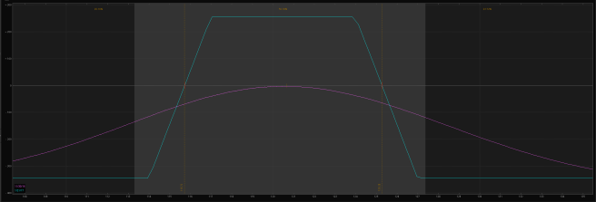
The executed trade payoff graph is shown below, where the blue line is payoff at expiry, the purple curved line is payoff right now, and the percent values at the top are probability zones. This graph can be made/found in the ToS Analyze tab.

That’s about it from start to finish. The GLD IC was put on with similar reasoning.

Today’s Trades (Greeks on Open):

1. STO 1 Jan17 TLT 114/117/124/127 IC @ $1.27
   • Delta: -0.36
   • Gamma: -3.05
   • Vega: -8.56
   • Theta: 1.11
2. STO 1 Jan17 GLD 103/106/118/121 IC @ $0.70
   • Delta: -0.85
   • Gamma: -2.68
   • Vega: -7.01
   • Theta: 0.95

The two trades have a combined buying power reduction (BPR) of $300 a piece, which is 12% of our account value per trade. This is higher than I’d like, but with a small account we’re in a tough place with putting on good trades while also keep our risk low.

In previous posts, I’ve talked a little bit about comparing implied volatility to historical/realized volatility as well as implied volatility to itself. That’s all well and good, but how do we go about actually doing it? I’m a very visual guy, so I cooked up a very simple indicator for my platform (TDA’s ThinkOrSwim) that allows us to see both comparisons cleanly in one window. All I did is take TastyTrade’s IV rank indicator and add the following to the beginning of the ThinkScript:

plot historical= reference historicalvolatility(45)*100;
historical.SetLineWeight(2);

When we put that all together, we get a very powerful study that shows us the current implied volatility compared to the 45 day historical volatility, as well as the current IV rank and IV percentile, which in different ways describe the implied volatility versus itself. I picked 45 days for the HV plot as it is halfway between the 30 and 60 day window I want to use for our options trades. Once you have this study set up, it’s trivial to change that window or add 5, 15 or 30 day HV plots to get a more thorough volatility picture.

Our charts for each of the 10 underlyings we picked earlier look like this:

The price chart is “naked,” meaning void of any technical indicators or S&R levels, and the bottom pane shows 45 day HV (blue line) vs implied volatility, which is colored green when elevated and red otherwise. This simple setup allows us to identify opportunities before we switch over to the options chain and start constructing trades.

In addition to the straight IV/HV and IV/IV comparisons, we will also look at volatility skew. Contrary to what many models predict, (implied) volatility is not the same across strike prices. If it was, we would expect to see a flat IV vs. Strike plot. Instead, we see the following plot for PG calls, which can be found in ToS under Charts–>Product Depth:

This shows us that ATM call IV is lower than OTM call IV, and much lower than ITM call IV. While not terribly interesting in and of itself, we can use these charts to examine when, for example, put IV is richer than call IV, and help us make the best trades given a general volatility assumption.

Between the options chain, our special IV vs. HV / IV vs. IV study, and IV curves, we now have everything we need to start identifying opportunities and placing trades.

Happy Thanksgiving, everyone! I’ve wrote a lot so far about how we will be trading volatility versus price action, and a natural question that might arise is what tools or indicators we will use to identify opportunities. Traders that look to exploit opportunities in price action such as scalpers and trend traders will often use technical support/resistance levels or indicators to make their trades. This is possible because price action behaves differently than volatility. I often hear people refer to instrument prices as “random,” and that’s only sort of true, and leaves out a lot of important subtlety. What is closer to the truth is that instrument returns are random, but even then not in the typical way we use the word “random.”

In literature as well as several popular options pricing models, returns are represented with a type of stochastic process called Geometric Brownian Motion. A stochastic process is one where the variable at time t (i.e. today’s return) is random but also partially dependent on the variable at time t-1 (yesterday’s return). If returns were truly random, with each discrete return being i.i.d., today’s return would have absolutely no effect on tomorrow’s. Anyone that has watched the market for more than a day knows this is not the case, but I will leave the proof as an exercise to my readers.

Volatility, on the other hand, exhibits much different behavior. While it is also often modeled stochastically, volatility exhibits a very special behavior that returns do not: clustering. All clustering means is that while we may see periods of elevated volatility, over time volatility tends to revert towards a long term mean. When people call volatility “mean-reverting,” this is what they are referring to. This clustering behavior is what allows us to trade volatility, and understanding it is crucial to cashing checks.

If we believe volatility clustering to be true, then we also believe that when volatility is especially elevated it will eventually revert to a long term mean. By extension, we also believe that when volatility is priced towards that long term mean, eventually we will see a cluster of higher volatility above that mean. This is the foundation of trading volatility.

As money transfers start to clear and we prepare to make our first trade, I felt it was important to make a post regarding directional assumptions. When laying on strategies that are typical delta neutral (e.g. iron condors, straddles, etc), there is often a temptation to skew the legs one way or the other because we think the underlying has room to run. This type of thinking is dangerous for two reasons. The first reason is that if we do have a directional assumption, meaning we believe the underlying is more likely to move one way than the other, we have better means to profit than a 4 legged spread. A credit or debit spread, or even a back or ratio spread, would be a better idea if we are so certain of a directional move. The second is that we will end up fighting the market. If the options market believes there is a stronger chance of the stock moving up (down), then calls (puts) will be richer. If we strive to maintain a mostly delta neutral portfolio, we should trade according to volatility and market greeks, not what we feel is that correct direction.

It’s ok to trade skew, and it’s something we will look at with each trade, but trying to fade moves with delta neutral strategies is a recipe for disaster, as reversals are typically already priced in to the options market.

I’m looking forward to placing our first trades next week. It might be tough as we move into the Christmas season when volatility and volume tends to fall off, but we’ll do our best to be smart and trade the market we’re given. Expect more frequent posts in the coming weeks.